In this tutorial, we will analyze an RNA sequencing (RNA-seq) dataset generated by Aldinger et al. from postmortem brain tissue of four female Rett syndrome patients and age-matched female controls (https://doi.org/10.1038/s41597-020-0527-2). This dataset is already integrated as an example dataset in the ArrayAnalysis app. Rett syndrome is a rare neurodevelopmental disorder caused by mutations in the X-linked MECP2 gene.
Start the analysis of the data by clicking "Start Analysis" after selecting "RNA-Seq Analysis" and "Raw count". In the next tab, click on "Run example".
After uploading the data, the metadata and a preview of the count table are shown. In the metadata, you can see that there are four experimental groups: the cingulate and temporal cortex of controls and the cingulate and temporal cortex of Rett syndrome patients. Each experimental group includes 4 samples.
16 and 31, respectively. You can find this answer by looking in the metadata tab at the data upload page. You can sort the metadata by age.
Proceed to the pre-processing step, by clicking "Next" (bottom left of the page) or by clicking the "pre-processing" tab at the navigation bar. In this step, you can remove samples, remove lowly expressed genes, and perform normalization. Select "Genotype" and "Tissue" as experimental group and start the data pre-processing by clicking on "Calculate".

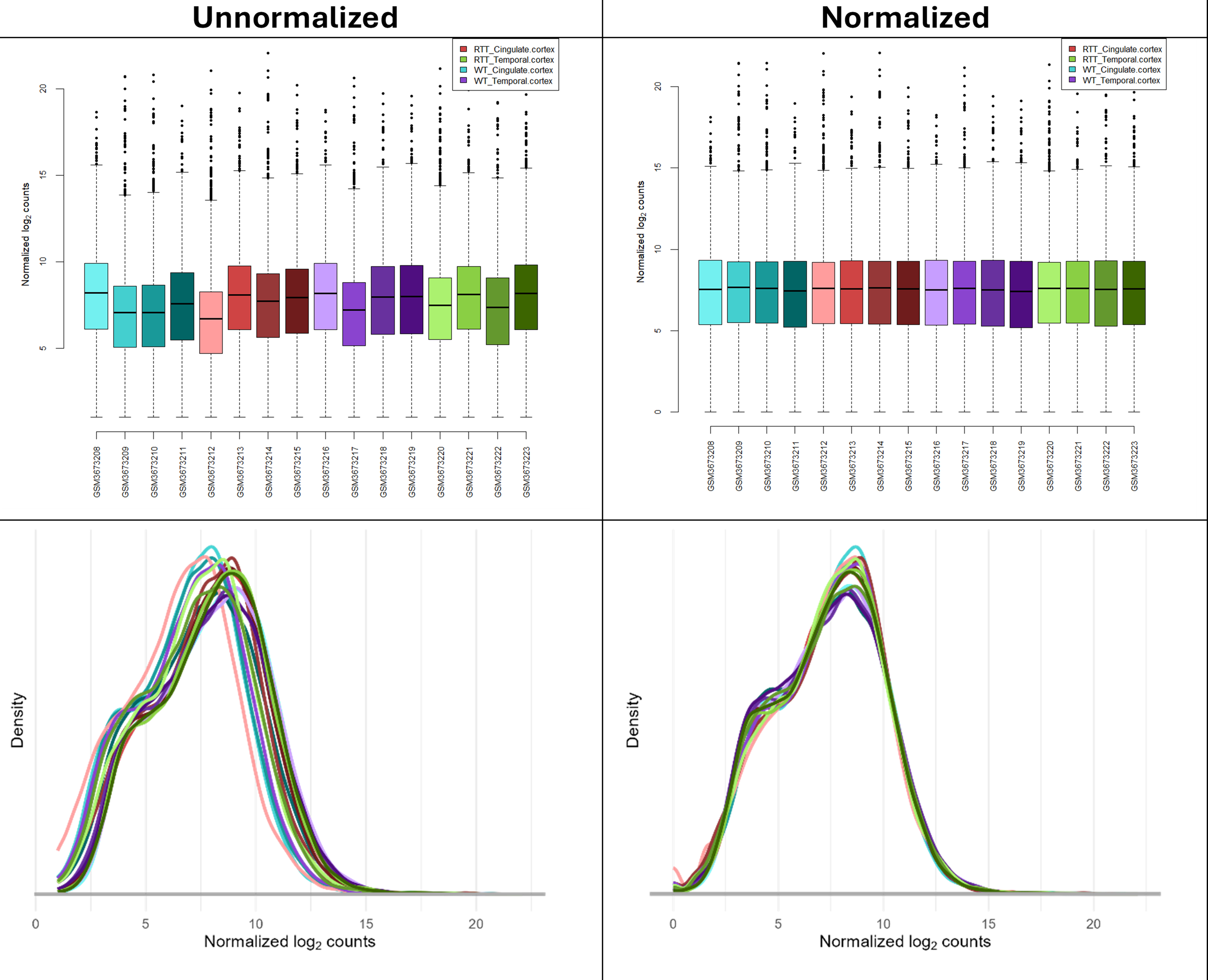
Normalization is needed to adjust for sample-to-sample variability and make the data comparable between samples. Without normalization the boxplots and density plots would show notable differences in the distribution between samples (see figure below).

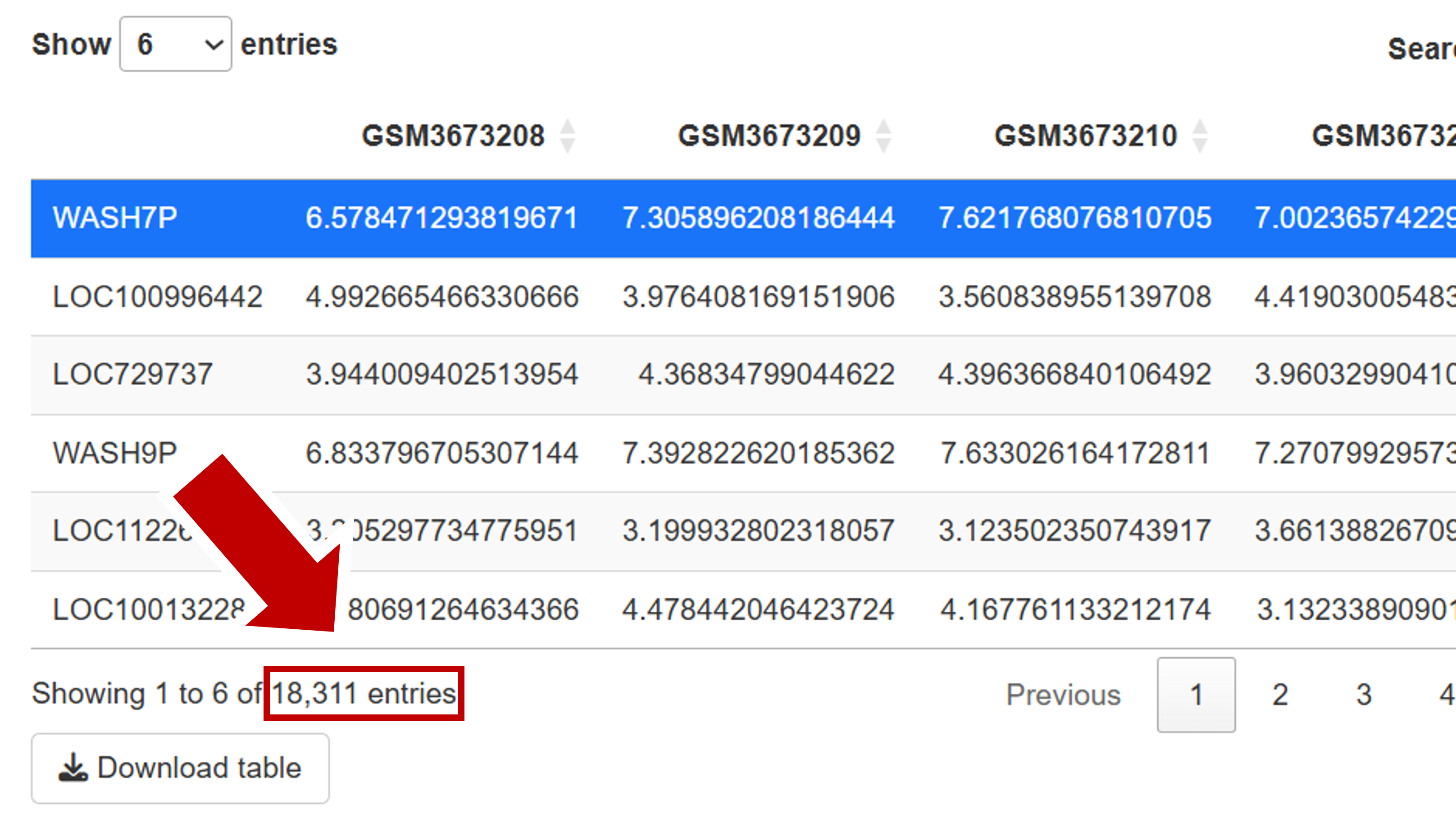
Filtering is needed to remove lowly expressed genes, where the measurements are subject to noise and which cannot be analyzed confidently. So, we filter for minimal expression levels (of 10 reads in at least a substantial subset of the samples). If you apply a threshold of 10, 18,311 genes passed the filtering (see bottom of normalized count table).

In the PCA plot and correlation plot, you can see that there seems to be some clustering by genotype (which would be expected), but the clustering is not perfect (two of the clear subclusters consist of one genotype only, one is mixed). Moreover, there is almost perfect clustering per patient (which may also be expected), but again not perfect (some samples of the same individual don’t cluster together for the two tissues studied).
After we have pre-processed the data, we want to compare the expression profiles of Rett syndrome patients with the controls in the temporal cortex. Furthermore, we would like to correct for age and add Ensembl IDs to the output. Please select the correct options on the statistical analysis page and click "Calculate".

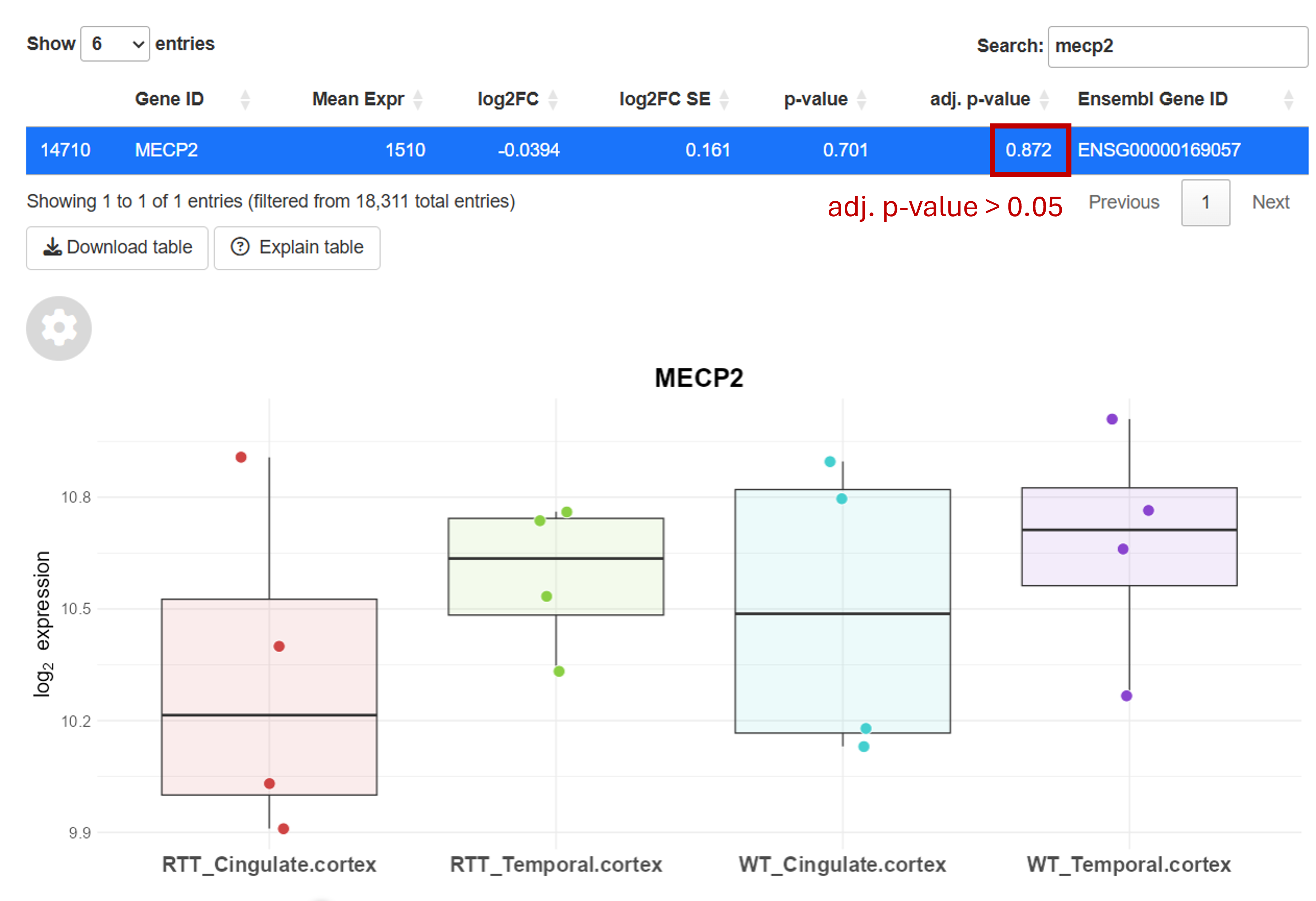
The adj. p-value is adjusted for multiple testing. If you test many genes, you will end up with many false positives if you do not correct the p-value. For instance, with a 5% significance level for each test, performing 10 tests raises the chance of at least one false positive to about 40%. Hence, the adj. p-value should be used to limit the number of false positives and find truly differentially expressed genes.
You can look up genes using the search bar (top right of top table). Here, you can see that MECP2 is not differentially expressed.

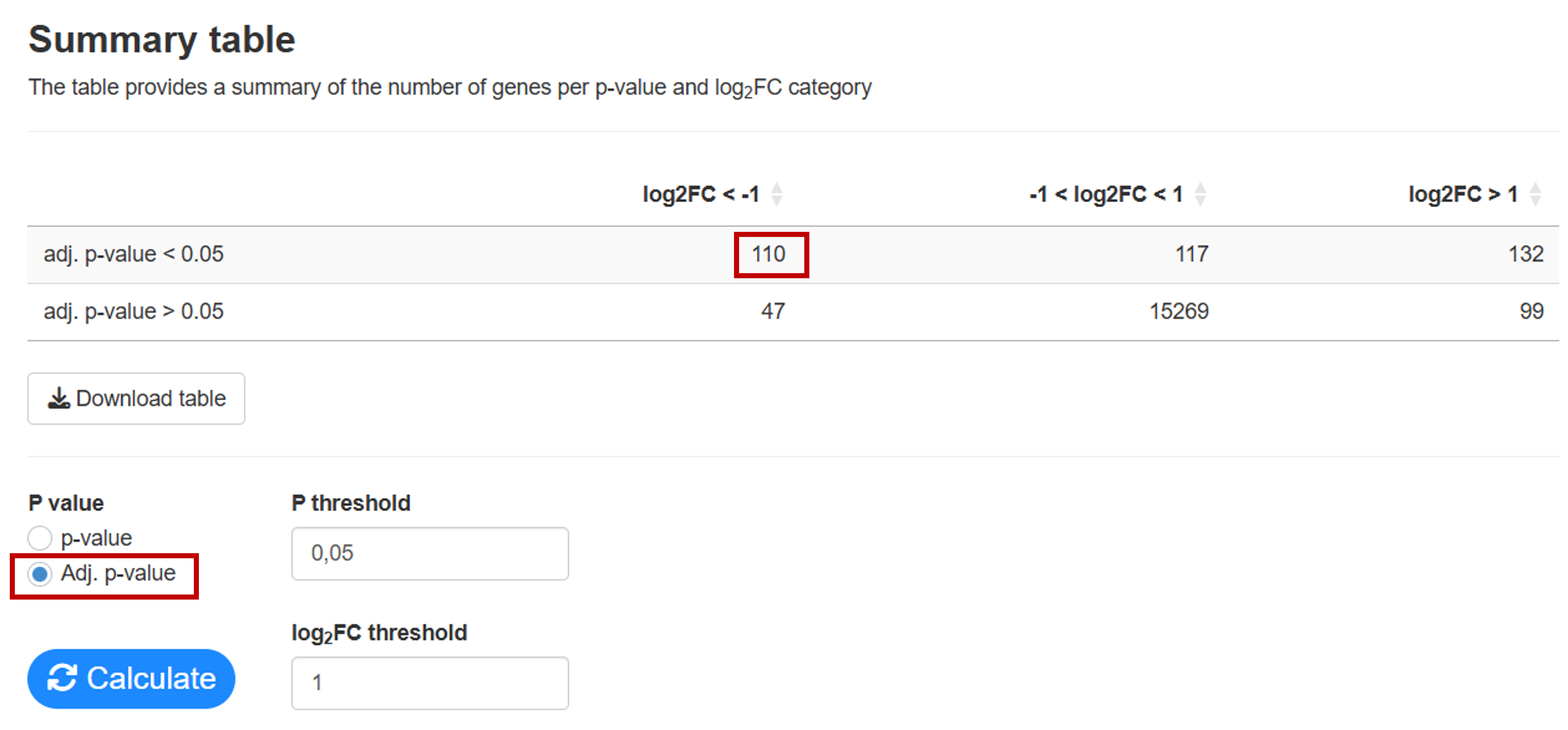
In the Summary tab you can calculate how many genes are up and downregulated for different p-value and log2FC thresholds. Here you can see that 110 genes are downregulated.

You can now perform gene set analysis to identify which biological processes and pathways are altered.
The exact processes and pathways will depend on which gene set collection is used and whether ORA or GSEA is performed. However, with both methods, you will find processes and pathways related to inflammation/immune response and synaptic signaling.